Route Optimization KPIs Every Logistics Leader Should Track

Tracking route optimization KPIs in logistics is the difference between running a delivery operation and understanding it. Most enterprises generate thousands of route plans each week and have no rigorous framework for measuring whether those routes are actually optimized. 

A retail chain managing 400 daily delivery zones can hit its aggregate cost targets and still be losing material margin per drop to inefficiencies that only surface at the route level.

Without the right KPIs, cost leakage, fleet underutilization, and missed delivery windows accumulate undetected until they appear in quarterly P&L reviews, by which point the patterns are months old and harder to trace.

The framework in this article covers cost efficiency, delivery performance, fleet utilization, sustainability, and AI-era metrics, complete with formulas, benchmarks, and a tiered dashboard architecture that connects route-level data to business outcomes. 

Locus’s AI-driven route optimization platform processes millions of route decisions for enterprises across retail, FMCG, and 3PL, and that operational perspective informs which KPIs actually move the needle.

Why Route Optimization Demands Its Own KPI Framework

DIFOT rates, inventory turns, and order accuracy ratios measure supply chain health at the aggregate level. None of them can tell a VP of Logistics whether a specific route plan generated above-average cost or whether a 3% rise in per-delivery spend last quarter was driven by route design, carrier rate changes, or volume mix. 

Route optimization becomes relevant in the intersection of cost control, service quality, and fleet efficiency, and measuring it well requires a KPI layer built for that specificity.

The gap becomes more pronounced as operations scale. A 3PL running 5,000 daily routes across four regions cannot evaluate whether last week’s fleet deployment was efficient if the only visibility is total spend and aggregate DIFOT. Missed delivery windows, high deadhead miles, and low vehicle fill rates can coexist with an acceptable aggregate cost-per-delivery number when the underlying route data is never examined.

AI-driven route optimization introduces variables that legacy KPI sets were not built to track. When routes change dynamically mid-execution based on live traffic, order cancellations, or driver delays, the relevant question shifts from “did we hit today’s plan” to “how well did the optimization layer respond to real-time conditions.” 

Dynamic rerouting generates reroute events, ETA recalculations, and exception triggers that have no equivalent in a warehouse metric or an inventory KPI. An effective measurement framework accounts for all of them.

Cost Efficiency KPIs That Reveal Route-Level ROI

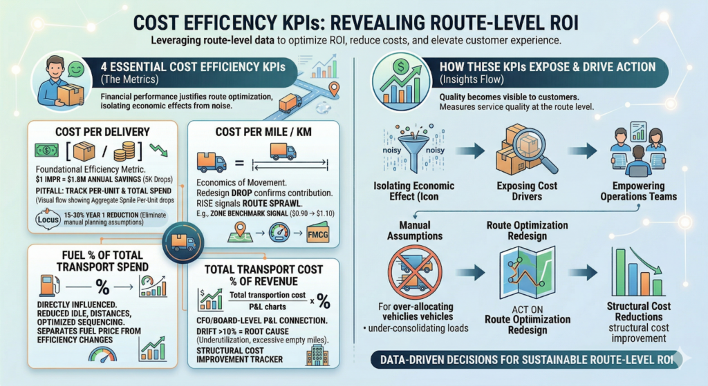
Financial performance is where route optimization either justifies itself or fails to. The cost KPIs below operate at the route level, isolating the economic effect of route planning decisions from the noise of carrier rate changes, fuel price swings, and volume shifts. Tracked consistently, they expose where cost is being generated and give operations teams the data needed to act on it.

Cost per delivery

Formula: Total delivery cost / Total successful deliveries

Cost per delivery is the foundational efficiency metric for any route optimization program. At enterprise scale, improving it by even $1 across 5,000 daily deliveries translates to $1.8 million in annual savings.

A common pitfall: cost per delivery can drop while total delivery spend rises, when volume increases faster than cost reduction. An operation that cut cost per delivery from $12 to $11 while scaling from 4,000 to 5,000 daily drops is spending more in aggregate despite the apparent improvement. Route optimization teams need to track both the per-unit figure and total spend in parallel rather than treating one as a substitute for the other.

Locus’s enterprise deployment data shows 15-30% delivery cost reductions in year one of implementation. The primary driver across clients is eliminating manual route planning assumptions that routinely over-allocate vehicles and under-consolidate loads.

Cost per mile and cost per kilometer

Formula: Total transportation cost / Total distance driven

Cost per mile strips volume effects from the efficiency picture and focuses directly on the economics of movement. A drop in cost per mile that coincides with a route redesign confirms the redesign’s contribution. An unexplained rise despite stable carrier rates typically signals route sprawl: routes covering more distance per stop than the plan intended.

For FMCG distributors replenishing retail stores on fixed cycles, cost per kilometer benchmarks by zone provide an early signal when route density is eroding. When a zone that historically ran at $0.90 per kilometer starts tracking at $1.10, the investigation starts with the route design.

Fuel cost as a percentage of total transportation spend

Formula: Total fuel spend / Total transportation cost x 100

Fuel represents a substantial share of transportation operating cost across all fleet types, and route optimization directly influences this ratio. Shorter total distances, reduced idle time, and optimized sequencing all reduce fuel burn per delivery. Tracking fuel as a percentage of transportation spend rather than as an absolute number separates the effect of fuel price changes from the effect of route efficiency changes over time.

Total transportation cost as a percentage of revenue

Formula: Total transportation cost / Total revenue x 100

The ratio connects route optimization directly to the P&L in a form that CFO-adjacent stakeholders recognize immediately. Enterprises that drift above 10% in this ratio frequently find that the root cause is in route planning: fleet underutilization, excessive empty miles, and unnecessary stop complexity all push the ratio upward. Tracking it quarterly against both internal targets and vertical benchmarks gives leadership teams a board-level indicator of whether route optimization programs are delivering structural cost improvement.

Delivery Performance KPIs That Tie Routes to Customer Experience

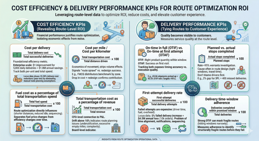
Delivery performance outcomes are where route planning quality becomes visible to customers. The KPIs below measure service quality at the route level, and improving them requires treating route design as a direct input to customer experience. 

The degree to which actual routes approximate the theoretical optimum, which routing efficiency measures directly, determines performance on every metric in this section more than driver behavior does.

On-time in full vs. on-time at first attempt

Two related but distinct KPIs often get conflated in logistics reporting.

• OTIF (On-Time In Full) measures whether the right product quantity arrived within the committed delivery window. To calculate on-time pickup performance: if 43 of 46 shipments were picked up on schedule, the rate is 93.5% (43 / 46 x 100). For top-quartile retail and FMCG operators, OTIF targets run at 95% or above.
  
• OTAF (On-Time At First Attempt) focuses on whether the delivery succeeded on the first visit. A delivery that arrives within the window but requires a second attempt because the recipient was unavailable registers as on-time under OTIF and as a failure under OTAF. Tracking both exposes whether the performance gap is in timing accuracy or delivery execution quality.

OTIF alone misleads without route deviation tracked alongside it. A route that consistently hits the delivery window only because drivers are running alternative roads accumulates extra distance, fuel cost, and vehicle wear that appear in other metrics. Route plan quality determines whether OTIF is achieved efficiently or expensively.

Planned vs. actual stops completed

Formula: Actual stops completed / Planned stops x 100

A stop completion rate below 95% warrants investigation at the route level. When drivers consistently complete fewer stops than planned, the cause is often in the route design: time windows set too tight, travel time underestimated, or stop-level service durations absent from the planning model. Blaming driver execution before examining the route plan produces the wrong corrective action.

The connection between planned stops and last-mile management is direct: for a 3PL managing high-density urban deliveries, a 2% gap in stop completion rate across 200 daily routes means 400 missed deliveries per day before any driver behavior analysis begins.

First-attempt delivery rate

Formula: First-attempt successful deliveries / Total delivery attempts x 100

Failed first attempts are among the most expensive outcomes in last-mile logistics. According to Locus’s operational data, for a company processing 10,000 daily orders, even a 5% increase in failed deliveries can result in an annual loss of $4.5 million. The re-delivery cycle adds driver time, fuel, dispatch overhead, and in high-SLA verticals, contractual penalties.

First-attempt delivery rate is partly a route planning problem. Time windows that don’t reflect recipient availability patterns, customer notification timing misaligned with ETA accuracy, and stop sequencing that places a business delivery at 6 PM are route decisions that produce first-attempt failures. Improving this rate requires examining the route plan as closely as the driver’s execution.

Delivery time-window adherence

Formula: Deliveries completed within promised window / Total deliveries x 100

An operation can post a strong OTIF number while window adherence flags that 15% of routes are hitting their windows by the narrowest of margins, meaning any disruption produces a miss. Measuring adherence at the route level identifies which routes are structurally fragile before they fail rather than after.

Fleet Utilization and Operational Efficiency KPIs

Fleet underutilization is the silent cost in route optimization. An operation running its fleet at 55% weight capacity and 60% cubic capacity per route can still post acceptable cost-per-delivery numbers while deploying 30-40% more vehicles than an optimized fleet would require for the same workload. The underutilization never surfaces in aggregate reports because the denominator adjusts with volume.

Vehicle utilization rate

Formula (weight): Actual load weight / Vehicle weight capacity x 100

Formula (volume): Actual load volume / Vehicle cubic capacity x 100

Vehicle utilization needs both dimensions. A route that fills a vehicle by weight but leaves 40% of cubic capacity unused is being planned against one constraint only. Carriers and 3PLs that fail to measure weight and volume utilization separately routinely underutilize fleet capacity in ways weight-only metrics never surface.

The impact of automated route planning on load consolidation is measurable: running both weight and volume constraints simultaneously during load assignment produces consolidation that manual dispatchers applying rules inconsistently cannot replicate at scale. A 4-point improvement in vehicle utilization across 200 daily routes typically translates to 12-15 fewer vehicles deployed each day.

Empty miles and deadhead percentage

Formula: Empty miles driven / Total miles driven x 100

Empty miles are the operational consequence of poor route sequencing and inadequate load consolidation. A vehicle completing its last delivery at a point far from its next loading location generates dead mileage that costs fuel and time without producing output.

Enterprises running mixed private and contracted fleets often see higher empty mile rates in contracted legs, where reverse logistics and backhaul opportunities are missed because planning happens per-trip rather than across the full route cycle. Route optimization applied to carrier assignment reduces this gap at the planning stage.

Truck turnaround time

Turnaround time measures the elapsed period from a vehicle’s departure from the hub to its return. Routes with long planned turnaround times that consistently exceed plan signal underestimated service times at stop level, dock scheduling constraints at specific customer locations, or load sequencing that forces drivers to resequence cargo at the stop.

Tracking turnaround against plan by route and zone reveals which areas of the network are structurally slower than planning assumptions, allowing route times and resource commitments to be recalibrated.

Stops per route and average route duration

Formula: Total route duration / Total routes completed

A decline in stops per route without a change in geographic territory signals route density loss. Average route duration trending above plan, without a corresponding rise in stops, signals inefficiency in sequencing or underestimated service times at specific stop types.

Sustainability and Emissions KPIs for Route Optimization

Sustainability KPIs have moved out of ESG reporting appendices and into operational dashboards. EU Corporate Sustainability Reporting Directive (CSRD) requirements now mandate scope 1 and scope 3 emissions disclosures for qualifying enterprises operating in Europe. EPA SmartWay requirements apply to logistics networks in the US freight sector. Major retailers are cascading carbon reduction targets to their 3PL partners as contractual terms. Measuring emissions at the route level is an operational requirement.

CO2 emissions per delivery and per kilometer

Formula (per delivery): Total route CO2 emissions / Total successful deliveries

Formula (per km): Total route CO2 emissions / Total kilometers driven

The two formulas give different insights. CO2 per delivery tracks carbon efficiency at the order level. CO2 per kilometer tracks the carbon intensity of movement, independent of delivery count. An operation expanding delivery density will see CO2 per delivery fall even as CO2 per kilometer holds steady. Tracking both prevents confusing density improvement with emissions reduction.

Route optimization reduces emissions through fewer total kilometers driven per delivery and reduced idle time at stop level through better sequencing. Locus’s enterprise clients have collectively avoided over 14 million kilograms of CO2 emissions, primarily through distance reduction and load consolidation across their delivery networks.

Fuel consumption per route

Formula: Total fuel consumed / Total routes completed

A route that consistently consumes 15-20% more fuel than comparably structured routes in the same zone is a redesign candidate. Tracking this per route rather than per fleet identifies where inefficiency is generating emissions above zone average.

Green routing compliance percentage

Formula: Routes meeting green routing constraints / Total routes planned x 100

Green routing constraints include low-emission zone entry restrictions (common across London, Paris, Amsterdam, and other European urban centers), EV range compliance for electric vehicle fleets, and time-of-day restrictions for diesel vehicles in specific urban areas. Measuring what share of planned routes comply with applicable green constraints before dispatch closes the gap between route planning quality and sustainability commitments.

How AI and Real-Time Data Are Redefining Route KPI Tracking

The fundamental difference between legacy KPI models and real-time orchestration models is when measurement happens. Traditional route optimization is batch-based: routes are planned in the morning, executed across the day, and analyzed in end-of-day reporting. KPIs under this model are retrospective by design, useful for identifying patterns and limited for preventing outcomes.

AI-driven orchestration changes the measurement requirement. When a platform dynamically reroutes based on live traffic, an order cancellation, or a driver running 20 minutes behind schedule, the relevant KPIs are live mid-execution signals that require real-time response. 

The enterprises operating at the top of OTIF and cost-per-delivery benchmarks are typically those with real-time KPI visibility connected to an automated tracking system that feeds route-level events back into operations as they occur.

Real-time plan-vs-actual route adherence

Plan adherence tracked at the route level in real time reveals which routes are deviating, by how much, and at which stage of execution. A driver who departs on schedule but begins diverging from the planned sequence at stop three is generating a signal that replanning tools can act on immediately, rerouting remaining stops to recover lost time before the delay compounds across the full route.

Reroute frequency and trigger analysis

Reroute frequency measures how often planned routes are revised mid-execution, and trigger analysis identifies why. High reroute frequency carries no inherent negative signal. It indicates the optimization layer is responding to real conditions. 

The diagnostic question is whether reroutes are being triggered by avoidable causes (poorly calibrated time windows, inaccurate traffic models) or genuine operational variance (weather, vehicle breakdowns, last-minute order additions).

Tracking trigger types alongside reroute frequency gives route planning teams the data to improve initial plan quality while measuring how effectively the AI layer handles unpredictable conditions.

Predictive ETA accuracy

Formula: Average of (Actual delivery time minus Predicted ETA) across all deliveries for a route or zone

ETA accuracy connects route planning quality to customer experience directly. A predicted ETA that drifts consistently by 25-30 minutes in a specific zone indicates a planning assumption requiring adjustment. Predictions staying within 10 minutes of actual arrival across 95%+ of deliveries reflect enterprise-grade accuracy. 

ETA accuracy also feeds exception management: when a predicted ETA crosses a delivery window threshold, operations teams can intervene before the miss occurs.

Exception rate per route

Formula: Routes with at least one exception event / Total routes completed x 100

Exception rate tracks the frequency of events requiring human intervention or automated replanning during execution. High exception rates on specific routes indicate structural planning problems, such as unrealistic time windows, poor stop sequencing, or geographic characteristics the planning model is not adequately accounting for.

Building an Enterprise Route Optimization KPI Dashboard

The value in route optimization measurement is rarely in tracking more KPIs. It is in structuring the right KPIs into a hierarchy that connects daily execution data to weekly operational decisions and quarterly strategic review. 

Enterprises that manage 20 KPIs with no prioritization framework act on noise rather than signal. The decision about which KPIs belong at which layer is where strategic route planning connects to measurement architecture.

The table below maps each KPI category to the appropriate review layer, audience, and primary action.

KPI layer	Review cadence	Primary audience	Primary KPIs	Resulting action
Strategic	Monthly and quarterly	VP Logistics, CFO, regional heads	Cost per delivery trend, transportation cost as % of revenue, total fleet CO2, OTIF by region	Network redesign, fleet investment, sustainability reporting
Tactical	Weekly	Operations managers, depot managers	Route deviation %, vehicle utilization by fleet class, empty miles %, stop completion rate	Route redesign, carrier reallocation, time window adjustment
Operational	Daily and real-time	Dispatch teams, supervisors	ETA accuracy, planned vs. actual stops, reroute trigger frequency, exception rate	Mid-execution intervention, same-day replanning

The clearest dividing line sits between the tactical and operational layers. Operations managers reviewing weekly data are identifying planning patterns to change. Dispatch teams reviewing real-time data are managing execution today. Mixing both audiences into a single dashboard view typically produces a report too granular for strategic decisions and too lagged for operational ones.

Strategic KPIs reviewed by leadership

Strategic KPIs belong in monthly or quarterly reviews with VP-level logistics leadership and the finance team. Cost per delivery trend lines, total fleet emissions by region, and OTIF performance across customer segments belong here. 

A retail chain with 15 regional distribution zones should track cost per delivery and OTIF independently by zone. A zone dragging the aggregate down by three to four points is a redesign candidate with a quantifiable ROI case attached to it.

Tactical KPIs reviewed weekly by operations managers

Route deviation percentage, vehicle utilization by fleet class, and empty miles percentage most reliably signal route planning quality at the operations manager level. 

A 5% week-over-week rise in empty miles for a specific depot needs investigation before it becomes a cost-per-delivery problem. Weekly cadence allows the team to identify the cause before the pattern becomes entrenched.

Operational KPIs monitored daily and in real time

ETA accuracy, planned versus actual stops, and reroute trigger frequency belong at this layer. Dispatch teams monitoring these metrics in real time can intervene before a delivery window miss occurs rather than logging it after the fact. Operations that invest in real-time visibility at this layer consistently post better OTIF performance than those relying on end-of-day reporting.

From KPI Measurement to KPI Improvement

Tracking the right KPIs is necessary. Converting measurement into improvement requires a way to connect KPI data to the planning decisions that generated it and a loop that feeds execution performance back into future route quality.

Benchmarking against internal history and industry averages

Benchmarking cost per delivery, vehicle utilization, and OTIF against internal historical data reveals where performance has changed and when. Benchmarking against industry averages identifies the gap between current performance and top-quartile operations in the same vertical. 

A retail logistics operation running at 82% vehicle utilization against a top-quartile benchmark of 88-90% has a measurable improvement case before examining any other metric.

How AI creates a feedback loop

AI-powered route optimization produces data about route performance that feeds back into the optimization model, improving future plan quality automatically. Every reroute event, every ETA deviation, and every exception trigger is a data point the algorithm draws from when building the next cycle of plans. 

The KPI data is an input to the next planning cycle and a reporting output from the last one simultaneously.

Timeline expectations for route optimization ROI

Locus’s operational data, drawn from enterprise deployments across retail, FMCG, and 3PL, shows measurable ROI materializing within 6-18 months of implementation. Route quality improvements surface first in cost per delivery and vehicle utilization, followed by delivery performance gains as time window accuracy improves.

Enterprises achieving top-quartile performance on these KPIs (99.5% OTIF, 15-30% cost reduction per delivery, sub-10% empty mile rates) are those that have moved from manual route planning to platform-driven execution with last-mile excellence built into the operational model.

Turn Route KPIs Into Continuous Performance Improvement

Knowing which KPIs to track is the starting point. Acting on them requires a system that surfaces route-level performance data in real time, connects those signals to dispatch decisions, and feeds execution data back into the optimization model automatically. 

The enterprises closing the gap between planned and actual performance on cost, delivery, fleet, and sustainability KPIs treat route optimization as a continuous measurement and improvement cycle.

Schedule a Locus demo to see how enterprise logistics teams are turning route optimization KPIs into automated, AI-driven performance improvements.